Matplotlib
![]()
import matplotlib.pyplot as plt
fig = plt.figure()
ax = fig.add_subplot(projection='3d')
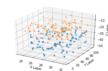
3D scatterplot
Demonstration of a basic scatterplot in 3D.
import matplotlib.pyplot as plt
import numpy as np

# Fixing random state for reproducibility
np.random.seed(19680801)

def randrange(n, vmin, vmax):
  """
  Helper function to make an array of random numbers having shape (n, )
  with each number distributed Uniform(vmin, vmax).
  """
  return (vmax - vmin)*np.random.rand(n) + vmin

fig = plt.figure()
ax = fig.add_subplot(projection='3d')

n = 100

# For each set of style and range settings, plot n random points in the box
# defined by x in [23, 32], y in [0, 100], z in [zlow, zhigh].
for m, zlow, zhigh in [('o', -50, -25), ('^', -30, -5)]:
  xs = randrange(n, 23, 32)
  ys = randrange(n, 0, 100)
  zs = randrange(n, zlow, zhigh)
  ax.scatter(xs, ys, zs, marker=m)

ax.set_xlabel('X Label')
ax.set_ylabel('Y Label')
ax.set_zlabel('Z Label')

plt.show()
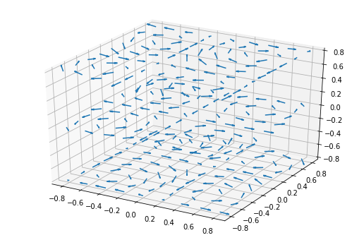
3D quiver plot
Demonstrates plotting directional arrows at points on a 3D meshgrid.
import matplotlib.pyplot as plt
import numpy as np

ax = plt.figure(figsize=(9, 6)).add_subplot(projection='3d')

# Make the grid
x, y, z = np.meshgrid(np.arange(-0.8, 1, 0.2),
             np.arange(-0.8, 1, 0.2),
             np.arange(-0.8, 1, 0.8))

# Make the direction data for the arrows
u = np.sin(np.pi * x) * np.cos(np.pi * y) * np.cos(np.pi * z)
v = -np.cos(np.pi * x) * np.sin(np.pi * y) * np.cos(np.pi * z)
w = (np.sqrt(2.0 / 3.0) * np.cos(np.pi * x) * np.cos(np.pi * y) *
     np.sin(np.pi * z))

ax.quiver(x, y, z, u, v, w, length=0.1, normalize=True)

plt.show()