Extended Kalman Filter Localization
import numpy as np
import math
import matplotlib.pyplot as plt
from scipy.spatial.transform import Rotation as Rot

Q = np.diag([
  0.1,  # variance of location on x-axis
  0.1,  # variance of location on y-axis
  np.deg2rad(1.0),  # variance of yaw angle
  1.0  # variance of velocity
]) ** 2  # predict state covariance

R = np.diag([1.0, 1.0]) ** 2  # Observation x,y position covariance

DT = 0.1  # time tick [s]
SIM_TIME = 50.0  # simulation time [s]

show_animation = True
Filter design
In this simulation, the robot has a state vector includes 4 states at time \(t\).
x, y are a 2D x-y position, \(\phi\) is orientation, and v is velocity.
In the code, “xEst” means the state vector. code
And, \(P_t\) is covariace matrix of the state,
\(Q\) is covariance matrix of process noise,
\(R\) is covariance matrix of observation noise at time \(t\)
x_state = np.array([0, 0, np.deg2rad(0), 2]).reshape(4,-1)
x_state
array([[0.],
       [0.],
       [0.],
       [2.]])
The robot has a speed sensor and a gyro sensor.
So, the input vecor can be used as each time step
Also, the robot has a GNSS sensor, it means that the robot can observe x-y position at each time.
The input and observation vector includes sensor noise.
def calc_input():
    v = 1.0  # [m/s]
    yawrate = 0.1  # [rad/s]
    u = np.array([[v], [yawrate]])
    return u

u = calc_input()
u
array([[1. ],
       [0.1]])
Motion Model
The robot model is
Given that
\(\textbf{x}_t = [x_t, y_t, \phi_t, v_t]\)
\(\textbf{x}_{t+1}\)
\(x_{t+1} = x_t + \dot{x}\Delta t\)
\(y_{t+1} = y_t + \dot{y}\Delta t\)
\(\phi_{t+1} = \phi_t + \dot{\phi}\Delta t\)
\(v_{t+1} = 0 + v_{t+1}\)
\(\textbf{u}_t = [v_t, \dot{\phi}]\)
So, the motion model is
where
\(\begin{equation*} F= \begin{bmatrix} 1 & 0 & 0 & 0\\ 0 & 1 & 0 & 0\\ 0 & 0 & 1 & 0 \\ 0 & 0 & 0 & 0 \\ \end{bmatrix} \end{equation*}\)
\(\begin{equation*} B= \begin{bmatrix} cos(\phi)\Delta t & 0\\ sin(\phi)\Delta t & 0\\ 0 & \Delta t\\ 1 & 0\\ \end{bmatrix} \end{equation*}\)
def motion_model(x, u, dt):
  F = np.array([[1.0, 0,  0,  0],
          [0,  1.0, 0,  0],
          [0,  0,  1.0, 0],
          [0,  0,  0,  0]])
  B = np.array([[dt * math.cos(x[2, 0]), 0 ],
          [dt * math.sin(x[2, 0]), 0 ],
          [0.0,            dt ],
          [1.0,            0.0]])
  x = F@x + B@u
  return x

# x = 0 + v_u*cos(0)*dt = 0.1
# y = 0 + v_u*sin(0)*dt = 0
# yaw = v_yaw * dt = 0.01
# v = v_u = 1
motion_model(x_state, u, DT)
array([[0.1 ],
       [0.  ],
       [0.01],
       [1.  ]])
Its Jacobian matrix is
\(\begin{equation*} J_F= \begin{bmatrix} \frac{dx}{dx}& \frac{dx}{dy} & \frac{dx}{d\phi} & \frac{dx}{dv}\\ \frac{dy}{dx}& \frac{dy}{dy} & \frac{dy}{d\phi} & \frac{dy}{dv}\\ \frac{d\phi}{dx}& \frac{d\phi}{dy} & \frac{d\phi}{d\phi} & \frac{d\phi}{dv}\\ \frac{dv}{dx}& \frac{dv}{dy} & \frac{dv}{d\phi} & \frac{dv}{dv}\\ \end{bmatrix} \end{equation*}\)
\(\begin{equation*} = \begin{bmatrix} 1& 0 & -v sin(\phi)dt & cos(\phi)dt\\ 0 & 1 & v cos(\phi)dt & sin(\phi) dt\\ 0 & 0 & 1 & 0\\ 0 & 0 & 0 & 1\\ \end{bmatrix} \end{equation*}\)
def jacob_f(x, u, DT):
  """
  Jacobian of Motion Model motion model
  """
  yaw = x[2, 0]
  v = u[0, 0]
  jF = np.array([
      [1.0, 0.0, -DT*v*math.sin(yaw), DT*math.cos(yaw)],
      [0.0, 1.0, DT*v*math.cos(yaw), DT*math.sin(yaw)],
      [0.0, 0.0, 1.0, 0.0],
      [0.0, 0.0, 0.0, 1.0]])

  return jF
Observation Model
The robot can get x-y position infomation from GPS.
Given that
\(\textbf{x}_t = [x_t, y_t, \phi_t, v_t]\)
\(\textbf{z}_t=[x_t,y_t]\)
So GPS Observation model is
where
\(\begin{equation*} H= \begin{bmatrix} 1 & 0 & 0& 0\\ 0 & 1 & 0& 0\\ \end{bmatrix} \end{equation*}\)
Its Jacobian matrix is
\(\begin{equation*} J_H= \begin{bmatrix} \frac{dx}{dx}& \frac{dx}{dy} & \frac{dx}{d\phi} & \frac{dx}{dv}\\ \frac{dy}{dx}& \frac{dy}{dy} & \frac{dy}{d\phi} & \frac{dy}{dv}\\ \end{bmatrix} \end{equation*}\)
\(\begin{equation*} = \begin{bmatrix} 1& 0 & 0 & 0\\ 0 & 1 & 0 & 0\\ \end{bmatrix} \end{equation*}\)
def observation_model(x):
  H = np.array([[1, 0, 0, 0],
          [0, 1, 0, 0]])
  z = H @ x
  return z

def jacob_h():
  # Jacobian of Observation Model
  jH = np.array([[1, 0, 0, 0],
           [0, 1, 0, 0]])
  return jH
Extented Kalman Filter
Localization process using Extendted Kalman Filter:EKF is
=== Predict ===
\(x_{Pred} = Fx_t+Bu_t\)
\(P_{Pred} = J_FP_t J_F^T + Q\)
=== Update ===
\(z_{Pred} = Hx_{Pred}\)
\(y = z - z_{Pred}\)
\(S = J_H P_{Pred}.J_H^T + R\)
\(K = P_{Pred}.J_H^T S^{-1}\)
\(x_{t+1} = x_{Pred} + Ky\)
\(P_{t+1} = ( I - K J_H) P_{Pred}\)
def ekf_estimation(xEst, PEst, z, u, dt):
  # Predict
  xPred = motion_model(xEst, u, dt)
  jF = jacob_f(xEst, u, dt)
  PPred = jF @ PEst @ jF.T + Q

  # Update
  jH = jacob_h()
  zPred = observation_model(xPred)
  y = z - zPred
  S = jH @ PPred @ jH.T + R
  K = PPred @ jH.T @ np.linalg.inv(S)
  xEst = xPred + K @ y
  PEst = (np.eye(len(xEst)) - K @ jH) @ PPred
  return xEst, PEst

xEst = np.zeros((4, 1)) # State Vector [x y yaw v]
PEst = np.eye(4) # Covariace matrix of the state
z = observation_model(xEst)
dt = 0.1  # time tick [s]
u = calc_input()
ekf_estimation(xEst, PEst, z, u, dt)
(array([[0.04950495],
        [0.        ],
        [0.01      ],
        [0.9950495 ]]),
 array([[0.5049505 , 0.        , 0.        , 0.04950495],
        [0.        , 0.5049505 , 0.04950495, 0.        ],
        [0.        , 0.04950495, 0.99535412, 0.        ],
        [0.04950495, 0.        , 0.        , 1.9950495 ]]))
# Simulation parameter
INPUT_NOISE = np.diag([1.0, np.deg2rad(30.0)]) ** 2
GPS_NOISE = np.diag([0.5, 0.5]) ** 2

def observation(xTrue, u, dt):
  xTrue = motion_model(xTrue, u, dt)

  # add noise to gps x-y
  z = observation_model(xTrue) + GPS_NOISE @ np.random.randn(2, 1)

  # add noise to input
  ud = u + INPUT_NOISE @ np.random.randn(2, 1)
  return xTrue, z, ud


xs_init = np.zeros((4,1))
u = calc_input()
xTrue, z, ud = observation(xs_init, u, dt=1)
xRaw = motion_model(xs_init, ud, dt=1)

print(xTrue)
print(xRaw)
print(z)
print(ud)
[[1. ]
 [0. ]
 [0.1]
 [1. ]]
[[2.31589188]
 [0.        ]
 [0.18290528]
 [2.31589188]]
[[1.46433487]
 [0.22398672]]
[[2.31589188]
 [0.18290528]]
def plot_covariance_ellipse(xEst, PEst):
  Pxy = PEst[0:2, 0:2]
  eigval, eigvec = np.linalg.eig(Pxy)

  if eigval[0] >= eigval[1]:
    bigind = 0
    smallind = 1
  else:
    bigind = 1
    smallind = 0

  t = np.arange(0, 2*math.pi + 0.1, 0.1)
  a = math.sqrt(eigval[bigind])
  b = math.sqrt(eigval[smallind])
  x = [a * math.cos(it) for it in t]
  y = [b * math.sin(it) for it in t]
  angle = math.atan2(eigvec[1,bigind], eigvec[0,bigind])
  rot = Rot.from_euler('z', angle).as_matrix()[0:2, 0:2]
  fx = rot @ (np.array([x,y]))
  px = np.array(fx[0,:] + xEst[0,0]).flatten()
  py = np.array(fx[1,:] + xEst[1,0]).flatten()
  plt.plot(px, py, "--r")
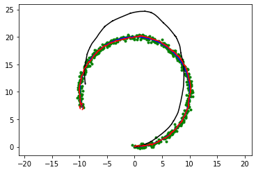
This is a sensor fusion localization with Extended Kalman Filter(EKF).
The blue line is true trajectory, the black line is dead reckoning trajectory,
the green point is positioning observation (ex. GPS), and the red line is estimated trajectory with EKF.
The red ellipse is estimated covariance ellipse with EKF.
from IPython import display

time = 0.0

# State Vector [x y yaw v]'
xEst = np.zeros((4, 1))
xTrue = np.zeros((4, 1))
PEst = np.eye(4)

xDR = np.zeros((4, 1))  # Dead reckoning

# history
hxEst = xEst
hxTrue = xTrue
hxDR = xTrue
hz = np.zeros((2, 1))

fig = plt.figure()
plt.axis("equal")
plt.grid(True)
while SIM_TIME >= time:
  time += DT
  u = calc_input()

  xTrue, z, ud = observation(xTrue, u, DT)
  xDR = motion_model(xDR, ud, dt=DT) # Only compute with ud
  xEst, PEst = ekf_estimation(xEst, PEst, z, ud, dt=DT)

  # store data history
  hxEst = np.hstack((hxEst, xEst))
  hxDR = np.hstack((hxDR, xDR))
  hxTrue = np.hstack((hxTrue, xTrue))
  hz = np.hstack((hz, z))

  if show_animation:
    plt.cla()
    # # for stopping simulation with the esc key.
    # plt.gcf().canvas.mpl_connect('key_release_event',
    #     lambda event: [exit(0) if event.key == 'escape' else None])
    plt.plot(hz[0,:], hz[1,:], ".g")
    plt.plot(hxTrue[0,:].flatten(),
         hxTrue[1,:].flatten(), "-b")
    plt.plot(hxDR[0,:].flatten(),
         hxDR[1,:].flatten(), "-k")
    plt.plot(hxEst[0,:].flatten(),
         hxEst[1,:].flatten(), "-r")
    plot_covariance_ellipse(xEst, PEst)

    display.display(fig)
    display.clear_output(wait=True)