Lidar with Rotation
![]()
import numpy as np
from scipy.spatial.transform import Rotation as sciR
基本知识
线速度
\(\omega\)为角速度(三维向量),\(r\)为旋转半径(三维向量),那么线速度为:
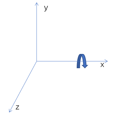
E.g.,假设IMU围绕x轴旋转,如果某点位于x轴上,此时该点旋转半径r和x轴重合,其线速度为0:
r = [1, 0, 0]
w = [2, 0, 0] # 逆时针为正,右手法则

np.cross(w, r)
array([0, 0, 0])
若某物体在该点\((1, 0, 0)\)的姿态和IMU姿态一致(即\(R\)为单位阵),其角速度应该等于IMU角速度:
R = np.eye(3, 3)
R @ w
array([2., 0., 0.])
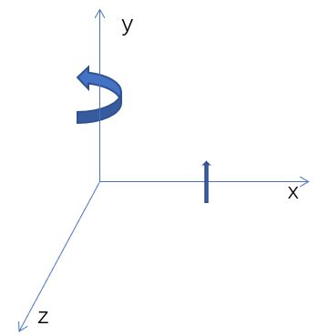
E.g.,假设IMU围绕y轴逆时针旋转,如果某点位于x轴上,其线速度方向应该为z轴的负方向:
r = [1, 0, 0]
w = [0, 2, 0]

np.cross(w, r)
array([ 0, 0, -2])
角速度和自身坐标系关系
角速度的积分得到的旋转向量\(\phi=\boldsymbol{\omega}_{k-1}\left(t_{k}-t_{k-1}\right)\)为\(t_k\)变换到\(t_{k-1}\)下的变换,而不需要求逆!因为此时是坐标系变换,等于参考向量被反向旋转。
例如IMU(坐标系)围绕自身x轴转90度(新x轴不变,新y轴为原来z轴,新z轴为原来-y轴),那么原来坐标系中的向量\([0, 1, 0]\)在新的坐标系下表示为\([0, 0, -1]\),对\([0, 0, -1]\)做变换看是否等于原向量\([0, 1, 0]\):
from scipy.spatial.transform import Rotation as sciR
R = sciR.from_rotvec(np.pi/2 * np.array([1, 0, 0]))

R.apply([0, 0, -1]).round()
array([ 0., 1., -0.])
汽车拐弯模拟
假设汽车以\(10 \text{m/s}\)速度和\(30^\circ \text{/s}\)角速度拐弯:
import matplotlib.pyplot as plt

w = np.array([0., 0., np.deg2rad(30)]) # 角速度
v = np.array([0., 10.0, 0.]) # 线速度 m/s
p = np.array([0., 0., 0.]) # 位置
dt = 0.01 # second

p_hst = [] # history of position
for i in range(300):
  R = sciR.from_rotvec(i*w*dt)
  p = p + R.inv().apply(v) * dt
  p_hst.append(p)
p_hst = np.array(p_hst)


plt.plot(p_hst[:, 0], p_hst[:, 1])
plt.xlim(0, 30)
plt.ylim(0, 30)
plt.show()

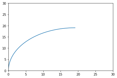
上面求当前旋转矩阵时是先求出相对\(t_0\)时刻转过的角度(\(w_1 \cdot \Delta t_1 + w_2 \cdot \Delta t_2 +\ ......\)),代码里假设了角速度和时间间隔不变:
R = sciR.from_rotvec(i*w*dt)
实际使用时应该采用积分形式,例如下面是旋转矩阵积分:
对应代码R = R * sciR.from_rotvec(w*dt)。
import matplotlib.pyplot as plt

w = np.array([0., 0., np.deg2rad(30)]) # 角速度
v = np.array([0., 10.0, 0.]) # 线速度 m/s
p = np.array([0., 0., 0.]) # 位置
dt = 0.01 # second

R = sciR.from_rotvec([0., 0., 0.])

p_hst = [] # history of position
for i in range(300):
  R = R * sciR.from_rotvec(w*dt)
  p = p + R.inv().apply(v) * dt
  p_hst.append(p)
p_hst = np.array(p_hst)


plt.plot(p_hst[:, 0], p_hst[:, 1])
plt.xlim(0, 30)
plt.ylim(0, 30)
plt.show()
4D雷达
雷达转动和位移的影响
Aqronos雷达扫描方式是4微秒一个点,所以点云是在时序上扫描得到的,对应一组连续的雷达坐标系。
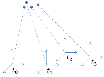
计算一个刚体的运动速度需要利用该刚体上多点的位置和速度信息,因此需要把所有的点转换到同一个坐标系中表示,这样各点的相对位置才准确。
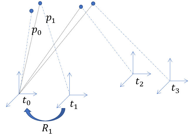
设三维空间中一个目标点在\(t_1\)时刻雷达坐标系下为\(\vec{p}_1\),将该点转换到\(t_0\)时刻雷达坐标系下为:
其中\(R_1\)为雷达坐标系\(t_1\)时刻相对\(t_0\)时刻的姿态,\(l\)为雷达位移。两边同时对求导可得:
其中\(\dot{R} = R \omega_{\times},\ (\omega \times \vec{a} = \omega_{\times}a)\)。
由于雷达测量点的速度\(v'_1\)为该点相对雷达的速度在雷达发射方向上的投影\(v'_1 = \vec{p}_1 \cdot \vec{v}_1\),带入上面公式可得:
由于\((\omega \times \vec{p}_1) \cdot \vec{p}_1 = 0\),而\((R_1^T\vec{v}_l) \cdot \vec{p}_1\)相当于汽车速度在雷达发射方向上的投影,移项得到:
同理可得其他点,并组成\(Ax = B\)的形式(这里假设雷达速度\(\vec{v}_l\)不发生变化):
def generatePoints(xc, yc, zc, n, xs=1, ys=1, zs=1):
  """
  @xc, yc, zc: points center
  @xs, ys, zs: points scale
  """
  points = np.random.rand(3, n)
  points[0] = points[0]*xs + xc
  points[1] = points[1]*ys + yc
  points[2] = points[2]*zs + zc
  return points

generatePoints(10, 50, 1, n=2)
array([[10.31871359, 10.2151918 ],
       [50.2594425 , 50.140402  ],
       [ 1.8613003 ,  1.40457554]])
Simulator:
from scipy.spatial.transform import Rotation as sciR

class Simulator:
  def __init__(self, w, v, vt, p, dt):
    self.w = w # 角速度
    self.v = v # 雷达速度
    self.vt = vt # 目标速度
    self.p = p # 雷达起始位置
    self.dt = dt # 间隔时间
    self.R = sciR.from_rotvec([0., 0., 0.]) # 单位阵

  @staticmethod
  def generateTargetPoints(xc, yc, zc, n, xs=1, ys=1, zs=1):
    """
    @xc, yc, zc: points center
    @xs, ys, zs: points scale
    """
    points = np.random.rand(3, n)
    points[0] = points[0]*xs + xc
    points[1] = points[1]*ys + yc
    points[2] = points[2]*zs + zc
    return points # shape: 3 x n

  def run(self):
    w = self.w # 角速度
    v = self.v # 雷达速度 m/s
    vt = self.vt # 目标速度 v-target
    p = self.p # 雷达起始位置
    dt = self.dt # second
    tps = self.tps # target points

    R = sciR.from_rotvec([0., 0., 0.])
    A = []
    B = []
    for i in range(len(self.tps)):
      R = R * sciR.from_rotvec(w*dt)
      p = p + R.inv().apply(v) * dt
      tp = tps[:, i] + vt*dt # target point
      p_t = tp - p
      A.append(R.apply(p_t))
      B.append(R.inv().apply(vt-v)@p_t)
    return A, B
w = np.array([0., 0., np.deg2rad(30)]) # 角速度
v = np.array([0., 10.0, 0.]) # 雷达速度 m/s
vt = np.array([2., 0., 5.]) # 目标速度 v-target
p = np.array([0., 0., 0.]) # 雷达起始位置
dt = 0.01 # second

Sim = Simulator(w, v, vt, p, dt)
Sim.tps = Simulator.generateTargetPoints(10, 50, 1, n=10) # target points

A, B = Sim.run()

print("gt:", vt)
print("estimation:", (np.linalg.pinv(A)@B + v).round(2))
gt: [2. 0. 5.]
estimation: [2. 0. 5.]
如果不考虑旋转,看下求解的目标速度和真值(gt)的误差情况:
# !pip install jdc
import jdc
%%add_to Simulator

def run_no_rotation(self):
  w = self.w # 角速度
  v = self.v # 雷达速度 m/s
  vt = self.vt # 目标速度 v-target
  p = self.p # 雷达起始位置
  dt = self.dt # second
  tps = self.tps # target points

  R = sciR.from_rotvec([0., 0., 0.])
  A = []
  B = []
  for i in range(len(self.tps)):
    R = R * sciR.from_rotvec(w*dt)
    p = p + R.inv().apply(v) * dt
    tp = tps[:, i] + vt*dt # target point
    p_t = tp - p
    A.append(p_t)
    B.append(R.inv().apply(vt-v)@p_t)
  return A, B
A, B = Sim.run_no_rotation()

print("gt:", vt)
print("estimation:", (np.linalg.pinv(A)@B + v).round(2))
gt: [2. 0. 5.]
estimation: [11.57 -2.18 11.27]
Sim.w = np.array([0., 0., np.deg2rad(30)]) # 角速度
Sim.v = np.array([0., 10.0, 0.]) # 雷达速度 m/s
Sim.vt = np.array([20., 30., 5.]) # 目标速度 v-target
Sim.dt = 0.00004 # 40us
A, B = Sim.run_no_rotation()

print("gt:", Sim.vt)
print("estimation:", (np.linalg.pinv(A)@B + Sim.v).round(3))
gt: [20. 30.  5.]
estimation: [20.133 29.97   5.084]
Sim.w = np.array([0., 0., np.deg2rad(30)]) # 角速度
Sim.v = np.array([0., 60.0, 0.]) # 雷达速度 m/s
Sim.vt = np.array([20., 30., 5.]) # 目标速度 v-target
Sim.dt = 0.00004 # 40us
A, B = Sim.run_no_rotation()

print("gt:", Sim.vt)
print("estimation:", (np.linalg.pinv(A)@B + Sim.v).round(3))
gt: [20. 30.  5.]
estimation: [20.215 29.951  5.138]
Sim.w = np.array([0., 0., np.deg2rad(10)]) # 角速度
Sim.v = np.array([0., 60.0, 0.]) # 雷达速度 m/s
Sim.vt = np.array([20., 30., 5.]) # 目标速度 v-target
Sim.dt = 0.00004 # 40us
A, B = Sim.run_no_rotation()

print("gt:", Sim.vt)
print("estimation:", (np.linalg.pinv(A)@B + Sim.v).round(3))
gt: [20. 30.  5.]
estimation: [20.072 29.984  5.046]
Sim.w = np.array([0., 0., np.deg2rad(30)]) # 角速度
Sim.v = np.array([0., 10.0, 0.]) # 雷达速度 m/s
Sim.vt = np.array([20., 30., 5.]) # 目标速度 v-target
Sim.dt = 0.001 # 1ms
A, B = Sim.run_no_rotation()

print("gt:", Sim.vt)
print("estimation:", (np.linalg.pinv(A)@B + Sim.v).round(3))
gt: [20. 30.  5.]
estimation: [23.385 29.235  7.141]
Sim.w = np.array([0., 0., np.deg2rad(30)]) # 角速度
Sim.v = np.array([0., 60.0, 0.]) # 雷达速度 m/s
Sim.vt = np.array([0., 0., 1.]) # 目标速度 v-target
Sim.dt = 0.001 # 1ms
A, B = Sim.run_no_rotation()

print("gt:", Sim.vt)
print("estimation:", (np.linalg.pinv(A)@B + Sim.v).round(3))
gt: [0. 0. 1.]
estimation: [ 2.711 -0.615  2.788]
Sim.w = np.array([0., 0., np.deg2rad(5)]) # 角速度
Sim.v = np.array([0., 60.0, 0.]) # 雷达速度 m/s
Sim.vt = np.array([0., 0., 1.]) # 目标速度 v-target
Sim.dt = 0.001 # 1ms
A, B = Sim.run_no_rotation()

print("gt:", Sim.vt)
print("estimation:", (np.linalg.pinv(A)@B + Sim.v).round(3))
gt: [0. 0. 1.]
estimation: [ 0.454 -0.103  1.299]
Sim.w = np.array([0., 0., np.deg2rad(5)]) # 角速度
Sim.v = np.array([0., 60.0, 0.]) # 雷达速度 m/s
Sim.vt = np.array([20., 70., 1.]) # 目标速度 v-target
Sim.dt = 0.005 # 5ms
A, B = Sim.run_no_rotation()

print("gt:", Sim.vt)
print("estimation:", (np.linalg.pinv(A)@B + Sim.v).round(3))
gt: [20. 70.  1.]
estimation: [26.439 68.541  5.152]
由于Aqronos雷达目标是逐行扫描(100ms/帧),如果总共20行,那么意味着上下两条线上点的间隔能差5ms。从上述仿真结果可以看出,即使雷达转动速度很低(5°/s),对目标速度方向求解有较大影响。