Unscented Kalman Filter¶

import math
import matplotlib.pyplot as plt
import numpy as np
from scipy.spatial.transform import Rotation as Rot
import scipy.linalg

Python Robotics¶

States and Control inputs¶

状态量：x坐标、y坐标、偏航角、速度

\(x\), \(y\) are a 2D x-y position, \(\phi\) is orientation, and \(v\) is velocity.

\(\textbf{x}_t=[x_t, y_t, \phi_t, v_t]\)

控制量：速度、角速度

The robot has a speed sensor and a gyro sensor.

\(\textbf{u}_t=[v_t, \omega_t]\)

def calc_input():
  v = 1.0  # [m/s]
  yawRate = 0.1  # [rad/s]
  u = np.array([[v, yawRate]]).T
  return u

u = calc_input()
u

array([[1. ],
       [0.1]])

Motion Model¶

The robot model is

\( \dot{x} = vcos(\phi)\)
\( \dot{y} = vsin((\phi)\)
\( \dot{\phi} = \omega\)

Given that \(\textbf{x}_t = [x_t, y_t, \phi_t, v_t]\)，\(\textbf{u}_t = [v_t, \dot{\phi}]\)

the motion model is

\(\textbf{x}_{t+1} = f(x_t, u_t)\)
\(\qquad = F\textbf{x}_t+B\textbf{u}_t\)

\(x_{t+1} = x_t + \dot{x}\Delta t\)
\(y_{t+1} = y_t + \dot{y}\Delta t\)
\(\phi_{t+1} = \phi_t + \dot{\phi}\Delta t\)
\(v_{t+1} = 0 + v_{t+1}\)

where

\(\begin{equation*} F= \begin{bmatrix} 1 & 0 & 0 & 0\\ 0 & 1 & 0 & 0\\ 0 & 0 & 1 & 0 \\ 0 & 0 & 0 & 0 \\ \end{bmatrix} \end{equation*}\)

\(\begin{equation*} B= \begin{bmatrix} cos(\phi)\Delta t & 0\\ sin(\phi)\Delta t & 0\\ 0 & \Delta t\\ 1 & 0\\ \end{bmatrix} \end{equation*}\)

def motion_model(x, u, dt):
  F = np.array([[1.0, 0, 0, 0],
          [0, 1.0, 0, 0],
          [0, 0, 1.0, 0],
          [0, 0, 0, 0]])

  B = np.array([[dt * math.cos(x[2]), 0],
          [dt * math.sin(x[2]), 0],
          [0.0, dt],
          [1.0, 0.0]])
  x = F@x + B@u
  return x

Observation Model¶

观测量：x坐标、y坐标

The robot has a GNSS sensor.

\(\textbf{z}_t = [x_t, y_t]\)

Given that \(\textbf{x}_t = [x_t, y_t, \phi_t, v_t]\), so the observation model is

\(\textbf{z}_{t} = H\textbf{x}_t\)

where

\(\begin{equation*} H= \begin{bmatrix} 1 & 0 & 0& 0\\ 0 & 1 & 0& 0\\ \end{bmatrix} \end{equation*}\)

def observation_model(x):
  H = np.array([[1, 0, 0, 0],
          [0, 1, 0, 0]])
  z = H @ x
  return z

x = np.ones((4, 1))
observation_model(x)

array([[1.],
       [1.]])

给观测量和控制量加上噪音：

\(\textbf{u}_d = \textbf{u} + \epsilon\)

\(\textbf{z} = H\textbf{x} + \delta\)

# Simulation parameter
INPUT_NOISE = np.diag([1.0, np.deg2rad(30.0)]) ** 2
GPS_NOISE = np.diag([0.5, 0.5]) ** 2

def observation(xTrue, u, dt):
  xTrue = motion_model(xTrue, u, dt)
  # add noise to gps x-y
  z = observation_model(xTrue) + GPS_NOISE @ np.random.randn(2, 1)
  # add noise to input
  ud = u + INPUT_NOISE @ np.random.randn(2, 1)
  return xTrue, z, ud

xTrue = np.zeros((4, 1))
u = calc_input()
xTrue, z, ud = observation(xTrue, u, dt=1)
print('xTrue:\n', xTrue)
print('\nz:\n', z)
print('\nu:\n', u)
print('\nu with noise:\n', ud)

xTrue:
 [[1. ]
 [0. ]
 [0.1]
 [1. ]]

z:
 [[ 1.22539845]
 [-0.11166166]]

u:
 [[1. ]
 [0.1]]

u with noise:
 [[0.3668484 ]
 [0.23745866]]

Sigma points¶

In this case, the functions \(f\) and \(h\) are not linear. UKF applies UT to performs the approximation with extracted points called ”Sigma points. Sigma points are computed using the matrix \(S\) which is defined from the covariance matrix, \(\Sigma_t\). \(S_i\) denotes the i-th colum of the matrix \(S\)

\[S = \sqrt{\Sigma_t}\]

We define the sigma points \(X_{i,t} \in X_t\) as follows:

\[\begin{split} X_{i, t}=\left\{\begin{array}{ll} =\mu_{t}, & i=0 \\ =\mu_{t}+\gamma S_{i}, & i=1, \ldots, N \\ =\mu_{t}-\gamma S_{i-N}, & i=N+1, \ldots, 2 N \end{array}\right. \end{split}\]

where \(N\) is the dimension of the state, and \(\gamma\) is computed by:

\[\gamma = \sqrt{N+\lambda}\]

\[\lambda = \alpha^{2}(N+\kappa) - N\]

\(\alpha, \kappa\) are two hyper-parameters (scaling parameters) of UKF.

def generate_sigma_points(xEst, PEst, gamma):
  sigma = xEst
  Psqrt = scipy.linalg.sqrtm(PEst) # PEst = Psqrt @ Psqrt
  n = len(xEst[:, 0])
  # Positive direction
  for i in range(n):
    sigma = np.hstack((sigma, xEst + gamma*Psqrt[:, i:i+1]))

  # Negative direction
  for i in range(n):
    sigma = np.hstack((sigma, xEst - gamma*Psqrt[:, i:i+1]))
  return sigma

N = 4
ALPHA = 0.001
KAPPA = 0

lambda_ = ALPHA ** 2 * (N + KAPPA) - N
gamma = math.sqrt(N + lambda_)

xEst = np.zeros((N, 1))
xTrue = np.zeros((N, 1))
PEst = np.eye(N)
sigma_points = generate_sigma_points(xEst, PEst, gamma)
sigma_points.shape # (N, 2N+1)

(4, 9)

Predication¶

And then, the sigma points are passed through the nonlinear function \(f\):

\[\bar{X} = f(X)\]

def predict_sigma_motion(sigma, u, dt):
  """
    Sigma Points prediction with motion model
  """
  for i in range(sigma.shape[1]):
    sigma[:, i:i+1] = motion_model(sigma[:, i:i+1], u, dt)
  return sigma

u = calc_input()
perdicted_points = predict_sigma_motion(sigma_points, u, 1)
perdicted_points.shape

(4, 9)

Here \(\bar{X}\) are transformed sigma points. Finally, the objective parameters \(\mu'\) and \(\Sigma'\) of resultant Gaussian are calculated using the unscented transform on the tranformed sigma points, \(\mu', \Sigma^\ =\ UT(\bar{X}, \omega_m, \omega_c, Q)\):

\[\mu^{\prime} = \sum_{i=0}^{2n} \omega_i^m \bar{X}_i\]

\[\Sigma^{\prime} = \sum_{i=0}^{2n} \omega_i^c \left(\bar{X}_i-\mu^{\prime}\right)\left(\bar{X}_i-\mu^{\prime}\right)^{T} + Q\]

where \(Q\) is Transition model convariance;

and \(\omega^m\) are weights used when the mean is computed:

\[\begin{split} w_i^m=\left\{\begin{array}{ll} & =\frac{\lambda}{N+\lambda} & i=0 \\ & =\frac{1}{2(N+\lambda)}, & i=1, \ldots, 2 N \end{array}\right. \end{split}\]

and \(\omega^c\) are weights used when the covariance of Gaussian is recovered:

\[\begin{split} w^c_i=\left\{\begin{aligned} &=\frac{\lambda}{N+\lambda}+\left(1-\alpha^{2}+\beta\right) & i=0 \\ &=\frac{1}{2(N+\lambda)}, & i=1, \ldots, 2 N \end{aligned}\right. \end{split}\]

# UKF Parameter
ALPHA = 0.001
BETA = 2
KAPPA = 0

# calculate weights
wm = [lambda_ / (lambda_ + N)]
wc = [(lambda_ / (lambda_ + N)) + (1 - ALPHA**2 + BETA)]
for i in range(2*N):
  wm.append(1.0 / (2*(N + lambda_)))
  wc.append(1.0 / (2*(N + lambda_)))

wm = np.array([wm])
wc = np.array([wc])
wm.shape, wc.shape

((1, 9), (1, 9))

Recall that:

\(\mu^{\prime} = \sum_{i=0}^{2n} \omega_{m}^{[i]} \bar{X}^{[i]}\)

\(\Sigma^{\prime} = \sum_{i=0}^{2n} \omega_{c}^{[i]}\left(\bar{X}^{[i]}-\mu^{\prime}\right)\left(\bar{X}^{[i]}-\mu^{\prime}\right)^{T}\)

# Covariance for UKF simulation
Q = np.diag([
    0.1,  # variance of location on x-axis
    0.1,  # variance of location on y-axis
    np.deg2rad(1.0),  # variance of yaw angle
    1.0  # variance of velocity
]) ** 2  # predict state covariance

def calc_sigma_covariance(x, sigma, wc, Pi):
  nSigma = sigma.shape[1]
  d = sigma - x[0:sigma.shape[0]]
  P = Pi
  for i in range(nSigma):
    P = P + wc[0, i] * d[:, i:i+1] @ d[:, i:i+1].T
  return P

xPred = (wm @ perdicted_points.T).T
PPred = calc_sigma_covariance(xPred, perdicted_points, wc, Q)
xPred.shape, PPred.shape

((4, 1), (4, 4))

Update¶

Kalman filters perform the update in measurement space. Thus we must convert the sigma points of the prior into measurements using the measurement function \(h\):

\[ Z = h(\bar{X}) \]

Then we compute the mean and covariance of these points using the unscented transform, \(\mu_z, P_z = UT(Z, w_m, w_c, R)\).

The \(z\) subscript denotes that these are the mean and covariance of the measurement sigma points.)

\[\begin{split}\begin{aligned} \mu_z &= \sum_{i=0}^{2n} w^m_i Z_i \\ P_z &= \sum_{i=0}^{2n} w^c_i{(Z_i-\mu_z)(Z_i-\mu_z)^\mathsf T} + R \end{aligned} \end{split}\]

where \(R\) is Measurement model covariance.

# Update
R = np.diag([1.0, 1.0]) ** 2  # Observation x,y position covariance

zSigmaPoints = observation_model(perdicted_points)
mu_z = (wm @ zSigmaPoints.T).T
P_z = calc_sigma_covariance(mu_z, zSigmaPoints, wc, R)

mu_z.shape, P_z.shape

((2, 1), (2, 2))

Next we compute the residual and Kalman gain. The residual of the measurement \(z\) is trivial to compute:

\[y = \mathbf z_m - \mu_z\]

To compute the Kalman gain we first compute the cross covariance of the state and the measurements, which is defined as:

\[P_{xz} = \sum_{i=0}^{2n} w^c_i(\bar{X}_i - \mu')(Z_i - \mu_z)^\mathsf T\]

And then the Kalman gain is defined as

\[K = P_{xz}P^{-1}_z\]

If you think of the inverse as a kind of matrix reciprocal, you can see that the Kalman gain is a simple ratio which computes:

\[K \approx \frac{P_{xz}}{P_z} \approx \frac{\text{belief in state}}{\text{belief in measurement}}\]

def calc_pxz(sigma, x, z_sigma, zb, wc):
  nSigma = sigma.shape[1]
  dx = sigma - x
  dz = z_sigma - zb[0:2]
  P = np.zeros((dx.shape[0], dz.shape[0]))

  for i in range(nSigma):
    P = P + wc[0, i] * dx[:, i:i+1] @ dz[:, i:i+1].T
  return P

y = z - mu_z
Pxz = calc_pxz(perdicted_points, xPred, zSigmaPoints, mu_z, wc)
K = Pxz @ np.linalg.inv(P_z)
y.shape, Pxz.shape, K.shape

((2, 1), (4, 2), (4, 2))

Finally, we compute the new state estimate using the residual and Kalman gain:

\[\mathbf x = \mu' + Ky\]

and the new covariance is computed as:

\[ \mathbf P = \Sigma' - KP_zK^{\mathsf T} \]

xEst = xPred + K @ y
PEst = PPred - K @ P_z @ K.T

xEst.shape, PEst.shape

((4, 1), (4, 4))

xTrue, xEst

(array([[0.],
        [0.],
        [0.],
        [0.]]), array([[ 0.93523919],
        [-0.07444109],
        [ 0.06277945],
        [ 1.        ]]))

Sum-up¶

This table compares the equations of the linear KF and UKF equations.

\[\begin{split}\begin{array}{l|l} \textrm{Kalman Filter} & \textrm{Unscented Kalman Filter} \\ \hline & \boldsymbol{\mathcal Y} = f(\boldsymbol\chi) \\ \mathbf{\bar x} = \mathbf{Fx} & \mathbf{\bar x} = \sum w^m\boldsymbol{\mathcal Y} \\ \mathbf{\bar P} = \mathbf{FPF}^\mathsf T+\mathbf Q & \mathbf{\bar P} = \sum w^c({\boldsymbol{\mathcal Y} - \mathbf{\bar x})(\boldsymbol{\mathcal Y} - \mathbf{\bar x})^\mathsf T}+\mathbf Q \\ \hline & \boldsymbol{\mathcal Z} = h(\boldsymbol{\mathcal{Y}}) \\ & \boldsymbol\mu_z = \sum w^m\boldsymbol{\mathcal{Z}} \\ \mathbf y = \mathbf z - \mathbf{Hx} & \mathbf y = \mathbf z - \boldsymbol\mu_z \\ \mathbf S = \mathbf{H\bar PH}^\mathsf{T} + \mathbf R & \mathbf P_z = \sum w^c{(\boldsymbol{\mathcal Z}-\boldsymbol\mu_z)(\boldsymbol{\mathcal{Z}}-\boldsymbol\mu_z)^\mathsf{T}} + \mathbf R \\ \mathbf K = \mathbf{\bar PH}^\mathsf T \mathbf S^{-1} & \mathbf K = \left[\sum w^c(\boldsymbol{\mathcal Y}-\bar{\mathbf x})(\boldsymbol{\mathcal{Z}}-\boldsymbol\mu_z)^\mathsf{T}\right] \mathbf P_z^{-1} \\ \mathbf x = \mathbf{\bar x} + \mathbf{Ky} & \mathbf x = \mathbf{\bar x} + \mathbf{Ky}\\ \mathbf P = (\mathbf{I}-\mathbf{KH})\mathbf{\bar P} & \mathbf P = \bar{\mathbf P} - \mathbf{KP_z}\mathbf{K}^\mathsf{T} \end{array}\end{split}\]

def ukf_estimation(xEst, PEst, z, u, wm, wc, gamma, dt):
  # Predict
  sigma = generate_sigma_points(xEst, PEst, gamma)
  perdicted_points = predict_sigma_motion(sigma, u, dt)
  xPred = (wm @ sigma.T).T
  PPred = calc_sigma_covariance(xPred, sigma, wc, Q)

  # Update
  zSigmaPoints = observation_model(sigma)
  mu_z = (wm @ zSigmaPoints.T).T
  P_z = calc_sigma_covariance(mu_z, zSigmaPoints, wc, R)
  Pxz = calc_pxz(perdicted_points, xPred, zSigmaPoints, mu_z, wc)
  K = Pxz @ np.linalg.inv(P_z)
  y = z - mu_z
  xEst = xPred + K @ y
  PEst = PPred - K @ P_z @ K.T

  return xEst, PEst

def setup_ukf(nx, ALPHA, BETA, KAPPA):
  lamb = ALPHA ** 2 * (nx + KAPPA) - nx
  # calculate weights
  wm = [lamb / (lamb + nx)]
  wc = [(lamb / (lamb + nx)) + (1 - ALPHA ** 2 + BETA)]
  for i in range(2 * nx):
      wm.append(1.0 / (2 * (nx + lamb)))
      wc.append(1.0 / (2 * (nx + lamb)))
  gamma = math.sqrt(nx + lamb)

  wm = np.array([wm])
  wc = np.array([wc])

  return wm, wc, gamma

def plot_covariance_ellipse(xEst, PEst):  # pragma: no cover
  Pxy = PEst[0:2, 0:2]
  eigval, eigvec = np.linalg.eig(Pxy)

  if eigval[0] >= eigval[1]:
    bigind = 0
    smallind = 1
  else:
    bigind = 1
    smallind = 0

  t = np.arange(0, 2 * math.pi + 0.1, 0.1)
  a = math.sqrt(eigval[bigind])
  b = math.sqrt(eigval[smallind])
  x = [a * math.cos(it) for it in t]
  y = [b * math.sin(it) for it in t]
  angle = math.atan2(eigvec[1, bigind], eigvec[0, bigind])
  rot = Rot.from_euler('z', angle).as_matrix()[0:2, 0:2]
  fx = rot @ np.array([x, y])
  px = np.array(fx[0, :] + xEst[0, 0]).flatten()
  py = np.array(fx[1, :] + xEst[1, 0]).flatten()
  plt.plot(px, py, "--r")

DT = 0.1  # time tick [s]
SIM_TIME = 50.0  # simulation time [s]

# Covariance for UKF simulation
Q = np.diag([
    0.1,  # variance of location on x-axis
    0.1,  # variance of location on y-axis
    np.deg2rad(1.0),  # variance of yaw angle
    1.0  # variance of velocity
]) ** 2  # predict state covariance
R = np.diag([1.0, 1.0]) ** 2  # Observation x,y position covariance

# UKF Parameter
ALPHA = 0.001
BETA = 2
KAPPA = 0

def main():
  nx = 4  # State Vector [x y yaw v]'
  xEst = np.zeros((nx, 1))
  xTrue = np.zeros((nx, 1))
  PEst = np.eye(nx)
  xDR = np.zeros((nx, 1))  # Dead reckoning

  wm, wc, gamma = setup_ukf(nx, ALPHA, BETA, KAPPA)

  # history
  hxEst = xEst
  hxTrue = xTrue
  hxDR = xTrue
  hz = np.zeros((2, 1))

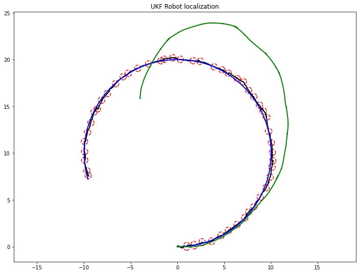
  plt.figure(figsize=(12,9))
  time = 0.0
  while SIM_TIME >= time:
    time += DT
    u = calc_input()

    xTrue, z, ud = observation(xTrue, u, DT)
    xDR = motion_model(xDR, ud, DT)

    xEst, PEst = ukf_estimation(xEst, PEst, z, ud, wm, wc, gamma, dt=DT)

    # store data history
    hxEst = np.hstack((hxEst, xEst))
    hxDR = np.hstack((hxDR, xDR))
    hxTrue = np.hstack((hxTrue, xTrue))
    hz = np.hstack((hz, z))
    if (int(time*10) % 10) == 0:
      plot_covariance_ellipse(xEst, PEst)

  plt.plot(hxEst[0, :], hxEst[1, :], color='k', lw=2)
  plt.plot(hxTrue[0, :], hxTrue[1, :], color='b', lw=2)
  plt.plot(hxDR[0, :], hxDR[1, :], color='g', lw=2)

  plt.axis('equal')
  plt.title("UKF Robot localization")
  plt.show()

main()

../_images/unscented_kalman_filter_30_0.png

cholesky VS sqrtm¶

正定矩阵 & 半正定矩阵¶

对于任意长度的非零向量\(X\)，若：

\(X^TAX > 0\)，则矩阵\(A\)为正定矩阵
\(X^TAX \ge 0\)，则矩阵\(A\)为半正定矩阵

记转换后的向量\(M = AX\)，则\(X^TAX = X^TM = \cos(\theta)\cdot ||M||\cdot||X||\)，那么意味着：

对于正定矩阵，\(\cos(\theta) > 0\)，即\(\theta < 90^{\circ}\)
对于半正定举证，\(\cos(\theta) \ge 0\)，即\(\theta \le 90^{\circ}\)

矩阵变换\(AX\)表示向量\(X\)会沿着该矩阵特征向量的方向进行变换（缩放），缩放比例由特征值\(\lambda\)决定。从特征值角度来看：

正定矩阵所有特征值都大于0
半正定矩阵所有特征值大于等于0

那么正定矩阵小于90度的含义是变换后的向量\(M\)是沿着原向量\(X\)的正方向进行缩放的（即\(M\)投影回原向量时方向不变）。

参考资料：

cholesky分解¶

Cholesky 分解是把一个对称正定的矩阵表示成一个下三角矩阵L和其转置的乘积的分解\(A = L L^T\)。它要求矩阵的所有特征值必须大于零，故分解的下三角的对角元也是大于零的。

A = np.array([[1, 0, 0],
        [1, 1, 1],
        [2, 1, 1]])

np.linalg.eig(A)[0]

array([2., 0., 1.])

由于\(A\)的特征值有0（半正定），所以不能用Cholesky分解，这里用sqrtm：

scipy.linalg.sqrtm(A) @ scipy.linalg.sqrtm(A)

array([[1., 0., 0.],
       [1., 1., 1.],
       [2., 1., 1.]])

再看下对称正定矩阵：

B = np.array([[6, -3, 1],
        [-3, 2, 0],
        [1, 0, 4]])

np.linalg.eig(B)[0]

array([7.81113862, 0.33192769, 3.85693369])

其特征值都大于0，那么可以用cholesky分解:

scipy.linalg.cholesky(B).T @ scipy.linalg.cholesky(B)

array([[ 6.00000000e+00, -3.00000000e+00,  1.00000000e+00],
       [-3.00000000e+00,  2.00000000e+00, -4.26642159e-17],
       [ 1.00000000e+00, -4.26642159e-17,  4.00000000e+00]])

filterpy¶

Kalman-and-Bayesian-Filters-in-Python中实现的filterpy。

!pip install filterpy

def motion_model(x, dt, u):
  F = np.array([[1.0, 0, 0, 0],
          [0, 1.0, 0, 0],
          [0, 0, 1.0, 0],
          [0, 0, 0, 0]])

  B = np.array([[dt * math.cos(x[2]), 0],
          [dt * math.sin(x[2]), 0],
          [0.0, dt],
          [1.0, 0.0]])
  x = F@x + B@u
  return x

def observation_model(x):
  H = np.array([[1, 0, 0, 0],
          [0, 1, 0, 0]])
  z = H @ x
  return z

def observation(xTrue, dt, u):
  # Simulation parameter
  INPUT_NOISE = np.diag([1.0, np.deg2rad(30.0)]) ** 2
  GPS_NOISE = np.diag([0.5, 0.5]) ** 2

  xTrue = motion_model(xTrue, dt, u)
  # add noise to gps x-y
  z = observation_model(xTrue) + GPS_NOISE @ np.random.randn(2)
  # add noise to input
  ud = u + INPUT_NOISE @ np.random.randn(2, 1)
  return xTrue, z, ud

from filterpy.kalman import MerweScaledSigmaPoints
from filterpy.kalman import UnscentedKalmanFilter as UKF

import numpy as np

dt = 0.1
sigmas = MerweScaledSigmaPoints(4, alpha=.001, beta=2., kappa=0)
ukf = UKF(dim_x=4, dim_z=2, fx=motion_model,
      hx=observation_model, dt=dt, points=sigmas)
ukf.x = np.zeros((4))

# Covariance for UKF simulation
ukf.Q = np.diag([
    0.1,  # variance of location on x-axis
    0.1,  # variance of location on y-axis
    np.deg2rad(1.0),  # variance of yaw angle
    1.0  # variance of velocity
]) ** 2  # predict state covariance
ukf.R = np.diag([1.0, 1.0]) ** 2  # Observation x,y position covariance


xTrue = np.zeros((4))
u = np.array([1, 0.1])
uxs = []
xs = []
for i in range(500):
  ukf.predict(u=u)
  xTrue, z, _ = observation(xTrue, dt, u)
  ukf.update(z)
  uxs.append(ukf.x.copy())
  xs.append(xTrue)
uxs = np.array(uxs).T
xs = np.array(xs).T

plt.figure(figsize=(12, 9))
plt.plot(uxs[0], uxs[1], color='k', lw=2, label='Estimated')
plt.plot(xs[0], xs[1], color='g', lw=2, label='True')
plt.axis('equal')
plt.title("UKF Robot localization")
plt.legend()
plt.show()

print(f'UKF standard deviation {np.std(uxs - xs):.3f} meters')

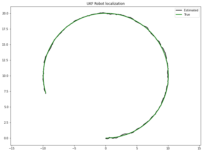
../_images/unscented_kalman_filter_43_0.png

UKF standard deviation 0.050 meters

Extended Kalman Filter Localization Path Planning

Austin's Notebook