KF Basics - Part I¶

#!pip install scipy

What is Expectation of a Random Variables?¶

Expectation is nothing but an average of the probabilites

\[\mathbb E[X] = \sum_{i=1}^n p_ix_i\]

In the continous form,

\[\mathbb E[X] = \int_{-\infty}^\infty x\, f(x) \,dx\]

import numpy as np
import random
x = [3, 1, 2]
p = [0.1, 0.3, 0.4]
E_x = np.sum(np.multiply(x, p))
print(E_x)

1.4000000000000001

Variance, Covariance and Correlation¶

Variance¶

Variance is the spread of the data. The mean does’nt tell much about the data. Therefore the variance tells us about the story about the data meaning the spread of the data.

\[\mathit{VAR}(X) = \frac{1}{n}\sum_{i=1}^n (x_i - \mu)^2\]

x = np.random.randn(10)
np.var(x)

1.140177413288341

Covariance¶

This is for a multivariate distribution. For example, a robot in 2-D space can take values in both x and y. To describe them, a normal distribution with mean in both x and y is needed.

For a multivariate distribution, mean $\mu$ can be represented as a matrix,

\[\begin{split} \mu = \begin{bmatrix}\mu_1\\\mu_2\\ \vdots \\\mu_n\end{bmatrix} \end{split}\]

Similarly, variance can also be represented.

But an important concept is that in the same way as every variable or dimension has a variation in its values, it is also possible that there will be values on how they together vary. This is also a measure of how two datasets are related to each other or correlation.

For example, as height increases weight also generally increases. These variables are correlated. They are positively correlated because as one variable gets larger so does the other.

We use a covariance matrix to denote covariances of a multivariate normal distribution: $$ \Sigma = \begin{bmatrix} \sigma_1^2 & \sigma_{12} & \cdots & \sigma_{1n} \\ \sigma_{21} &\sigma_2^2 & \cdots & \sigma_{2n} \\ \vdots & \vdots & \ddots & \vdots \\ \sigma_{n1} & \sigma_{n2} & \cdots & \sigma_n^2 \end{bmatrix} $$

Diagonal - Variance of each variable associated.

Off-Diagonal - covariance between $i$th and $j$th variables.

\[\begin{split}\begin{aligned}VAR(X) = \sigma_x^2 &= \frac{1}{n}\sum_{i=1}^n(X - \mu)^2\\ COV(X, Y) = \sigma_{xy} &= \frac{1}{n}\sum_{i=1}^n[(X-\mu_x)(Y-\mu_y)\big]\end{aligned}\end{split}\]

Covariance taking the data as sample with $\frac{1}{N-1}$

x_cor = np.random.rand(1,10)
y_cor = np.random.rand(1,10)
np.cov(x_cor, y_cor)

array([[0.11144314, 0.03499291],
       [0.03499291, 0.06883689]])

Covariance taking the data as population with $\frac{1}{N}$

np.cov(x_cor, y_cor, bias=1)

array([[0.10029882, 0.03149362],
       [0.03149362, 0.0619532 ]])

Gaussians¶

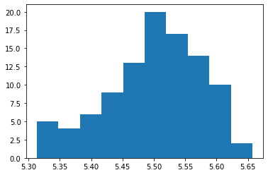
Central Limit Theorem¶

According to this theorem, the average of n samples of random and independent variables tends to follow a normal distribution as we increase the sample size. (Generally, for n>=30)

import matplotlib.pyplot as plt
import random
a = np.zeros((100,))
for i in range(100):
    x = [random.uniform(1,10) for _ in range(1000)]
    a[i] = np.sum(x,axis=0) / 1000
plt.hist(a)
# plt.show()

(array([ 5.,  4.,  6.,  9., 13., 20., 17., 14., 10.,  2.]),
 array([5.31327274, 5.34767731, 5.38208188, 5.41648645, 5.45089102,
        5.4852956 , 5.51970017, 5.55410474, 5.58850931, 5.62291388,
        5.65731845]),
 <a list of 10 Patch objects>)

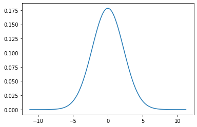
Gaussian Distribution¶

A Gaussian is a continuous probability distribution that is completely described with two parameters, the mean ($\mu$) and the variance ($\sigma^2$). It is defined as:

\[ f(x, \mu, \sigma) = \frac{1}{\sigma\sqrt{2\pi}} \exp\big [{-\frac{(x-\mu)^2}{2\sigma^2} }\big ] \]

Range is $$[-\inf,\inf] $$

This is just a function of mean($\mu$) and standard deviation ($\sigma$) and what gives the normal distribution the charecteristic bell curve.

import matplotlib.mlab as mlab
import math
import scipy.stats

mu = 0
variance = 5
sigma = math.sqrt(variance)
x = np.linspace(mu - 5*sigma, mu + 5*sigma, 100)
plt.plot(x, scipy.stats.norm.pdf(x,mu,sigma))
plt.show()

Gaussian Properties¶

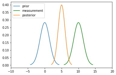
Multiplication

For the measurement update in a Bayes Filter, the algorithm tells us to multiply the Prior $P(X_t)$ and measurement $P(Z_t|X_t)$ to calculate the posterior:

\[P(X \mid Z) = \frac{P(Z \mid X)P(X)}{P(Z)}\]

Here for the numerator, $P(Z \mid X),P(X)$ both are gaussian.

$N(\mu_1, \sigma_1^2)$ and $N(\mu_2, \sigma_2^2)$ are their mean and variances.

New mean is

\[\mu_\mathtt{new} = \frac{\mu_1 \sigma_2^2 + \mu_2 \sigma_1^2}{\sigma_1^2+\sigma_2^2}\]

New variance is $$\sigma_\mathtt{new} = \frac{\sigma_1^2\sigma_2^2}{\sigma_1^2+\sigma_2^2}$$

import matplotlib.mlab as mlab
import math
import scipy.stats
mu1 = 0
variance1 = 2
sigma = math.sqrt(variance1)
x1 = np.linspace(mu1 - 3*sigma, mu1 + 3*sigma, 100)
plt.plot(x1, scipy.stats.norm.pdf(x1, mu1, sigma), label='prior')

mu2 = 10
variance2 = 2
sigma = math.sqrt(variance2)
x2 = np.linspace(mu2 - 3*sigma, mu2 + 3*sigma, 100)
plt.plot(x2, scipy.stats.norm.pdf(x2, mu2, sigma), "g-", label='measurement')

mu_new = (mu1*variance2 + mu2*variance1) / (variance1 + variance2)
print("New mean is at: ",mu_new)
var_new = (variance1*variance2)/(variance1+variance2)
print("New variance is: ",var_new)
sigma = math.sqrt(var_new)
x3 = np.linspace(mu_new - 3*sigma, mu_new + 3*sigma, 100)
plt.plot(x3, scipy.stats.norm.pdf(x3, mu_new, var_new), label="posterior")
plt.legend(loc='upper left')
plt.xlim(-10,20)
plt.show()

New mean is at:  5.0
New variance is:  1.0

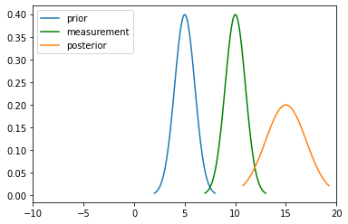
Addition

The motion step involves a case of adding up probability (Since it has to abide the Law of Total Probability). This means their beliefs are to be added and hence two gaussians. They are simply arithmetic additions of the two.

\[\begin{split}\begin{gathered}\mu_x = \mu_p + \mu_z \\ \sigma_x^2 = \sigma_z^2+\sigma_p^2\, \end{gathered}\end{split}\]

import matplotlib.mlab as mlab
import math
mu1 = 5
variance1 = 1
sigma = math.sqrt(variance1)
x1 = np.linspace(mu1 - 3*sigma, mu1 + 3*sigma, 100)
plt.plot(x1,scipy.stats.norm.pdf(x1, mu1, sigma), label='prior')

mu2 = 10
variance2 = 1
sigma = math.sqrt(variance2)
x2 = np.linspace(mu2 - 3*sigma, mu2 + 3*sigma, 100)
plt.plot(x2, scipy.stats.norm.pdf(x2, mu2, sigma), "g-", label='measurement')

mu_new = mu1 + mu2
print("New mean is at: ",mu_new)
var_new = (variance1+variance2)
print("New variance is: ",var_new)
sigma = math.sqrt(var_new)
x3 = np.linspace(mu_new - 3*sigma, mu_new + 3*sigma, 100)
plt.plot(x3, scipy.stats.norm.pdf(x3, mu_new, var_new),label="posterior")
plt.legend(loc='upper left')
plt.xlim(-10, 20)
plt.show()

New mean is at:  15
New variance is:  2

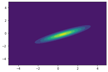
2D Gaussians¶

See bivariate Gaussian distribution for more details.

from scipy.stats import multivariate_normal
x, y = np.mgrid[-5:5:.1, -5:5:.1]
pos = np.empty(x.shape + (2,))
pos[:, :, 0] = x
pos[:, :, 1] = y
rv = multivariate_normal([0.5, -0.2], [[2.0, 0.9], 
                      [0.9, 0.5]])
plt.contourf(x, y, rv.pdf(pos))
plt.show()

Austin's Notebook